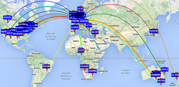
There’s something very nice with Raspberry Pi (RPi) is that you can use it’s GPIO output capability and somewhat precise clock to generate radio signals, especially weak signals radio signals (WSPR). These weak signals can travel thousands of kilometers and be received by foreign stations across the ocean. (No we’re not talking about receiving these radio signals with RTL-SDR, even though it’s nice too).
HAM License prerequisite… is not so bad
You need to have a HAM (Radio Amateur) license to transmit (yes, even a few milli-Watts (mW) or radiated power), but good news is that it’s the best time right now to pass your HAM license:
- France has just changed its license test method so that bad answer don’t cost you points, and you can repeat (cram) exams so it’s not that difficult.
- US has a much better and more progressive license scheme (Technician -> General -> Amateur Extra) and excellent teaching resources that makes it so much easier to get started.
- … and you’ve got plenty of time to prepare for exams since you can’t get out due to this covid-19 lockdown 🙂
Now if you look at the picture above, there’s a little circuit between the RPi and the antenna… why is that?
On being clean…
Well, the RPi was never intended to directly output radio signal, so it generates a square wave with plenty of harmonics (unwanted frequencies above the desired generated radio frequencies) that pollute the spectrum if you connect the RPi output directly to the antenna.
NOTE:
Having the privilege of sending radio waves worlwide comes with some small obligation: send clean radio signals! Don’t hurt your neighbour communications! Don’t force governments and regulators to limit our radio spectrum freedoms because we couldn’t self regulate. So far, HAM enthusiasts have done a great job not killing our radio passion. If you join, or plan on joining, please do the same.
Available Filters
So there are plenty of designs to make this output clean:
- TAPR WSPR RPI Hats that work with their RPi OS image to transmit on various frequencies (20m wavelength (14 MHz): 14.070 MHz – 14.350 MHz for weak signal digital communications, 30m (10MHz): 10.130 – 10.150 MHz for weak signal digital communications, 40m (7MHz)).
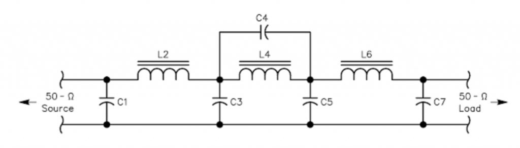
- DIY Designs that also include amplifiers, going past the few mW of RPi to a booming 1W !!! (see schematic below)
- Etc..

DIY Filter
Now the goal of experimentation is to learn by yourself and make your own stuff, so below is the documentation of a design in progress (fun in progress? some people will call us crazy) of a custom filter, by non-electronicians, for the RPi. (You’ll see that we go slowly and step by step over the process we used, so that it’s easy to follow and reproduce).
The goal of this filter is to:
- Learn about filters and electronic and RF,
- work on 7 MHz,
- for WSPR low signal (therefore low power, therefore we can maybe use some components such as Axial Fixed Inductors that are only for 0.25 W or 0.5W or 1W),
- be built with low part number,
- low complexity,
- with easy to procure and to solder electronic components: no or low CMS, no exotic part numbers, no need to print a PCB mandatorily…
- if possible no coil-winding (building the inductive coils),
- if possible with protection of the RPi from static electricity coming from the antenna.
- work on the RPi Zero W.
Actually, the goal of this post is to discuss between passionate individuals and critique the filter design(s) presented here, rather than providing a clean design.
So if you’re expecting a clean, profesionnal, working filter, this is maybe not the place.
Also, the goal is to document the (rather numerous) f..k-ups and mistakes we’ve done along the way, with their associated lessons-learned:
- Using RC filter: originally selected because it is announced as the simplest filters, it worked but was extremely low-power output, due to to the very nature of Resistive-Capacitive (RC) filters, yeah, it resists and dissipates heat, therefore weakening to radio output power… logical.. Replace with Inductive Capacitive (LC) filter.
- Using bread board: it is easy and fast, BUT bad for RF circuits because it can generate a lot of RF noise and doesn’t consistently provide a good grounding. Replace with copper-plate solder circuits.
A filter for an Antenna
RPi can generate radio signals for a variety of bands, up to the FM band (around 100 MHz radio signal). This means that you have quite a lot of HAM bands (Legacy or WARC) you can use. The lower the HAM radio frequency, the bigger the antenna, the farther you can expect it to go: HF (3 MHz-30 MHz) can travel across oceans, VHF (30 MHz-300MHz) – UHF (300 MHz – 3000 MHz or 3GHz) range is only a few kilometers in usual conditions.
Usually antennas are one fourth or half the wavelength, so if you’re operating on 7 MHz, the 40 m band, you can expect your antenna to be from 10 meters to 20 meters wide, or high, or both.
That means that you usually choose your operating frequency based on the space you have. Typically, in cities, you will probably choose higher frequencies with smaller antennas.
And based on your antenna, you will pick a filter that is allowing only frequencies for this antenna to exit the RPi and go to the antenna.
Building an antenna is a lot of fun, and antennas are so varied, up to the ones that enable you to receive from and transmit to a satellite. It’s much easier than you initially think. We’ll have plenty of episodes related to antenna building.
So let’s build a filter… and please give us feedback
There are many types of filters, as stated earlier. We started with a RC filter but the drop in desired radio signal output power was too important, therefore prompting to choose another filter, an LC filter that should preserve better the desired radio signal power and still be somewhat simple to build with common components.
Of these LC filters, we choose a Butterworth pass-band filter, for its apparent simplicity. Critique is welcome.
Pass band means that only one range of frequency can go through. It’s opposed to Low-Pass Filters (LPF: Only frequency below the cut-off frequency can go through) or High-Pass Filters (only frequencies above the cut-off frequency can go through the filter).
Filter design with Open Source
To design our Filter, we heard that QUCS open source software is handy and enables design from a library of filters and simulation of the filter. Actually we built and installed the MacOS version, with a few commands modification:
$ brew tap guitorri/tap$ brew tap cartr/qt4$ brew install qucs$ brew link qucs
Regarding installation on Linux, qucs was not in the APT packages of RPi. That’s because its Debian package was abandoned a few years ago. A lab member successfully compiled it using the official qucs wiki page on an AMD64 Debian 9 though, so there’s hope it might works on most distributions.
After this, we launch QUCS:
$ qucs &
First fun is that QUCS runs but isn’t launched in the foreground, you need to Alt-Tab or Command-Tab to select its icon to see its window (otherwise you spend a good amount of time saying “wow… must be super awesome large software that takes ages to start… really long… such 31337 software…”. actually QUCS is quite quick to launch!):
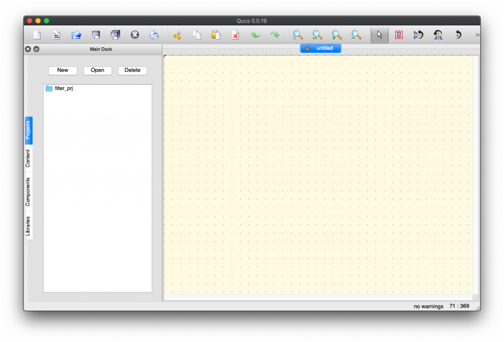
Then you can (and should) create a new project by Clicking “New” in the “Projects” side tab (here already created as you already see filter_prj).
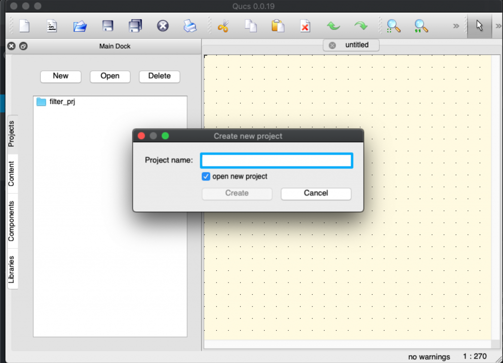
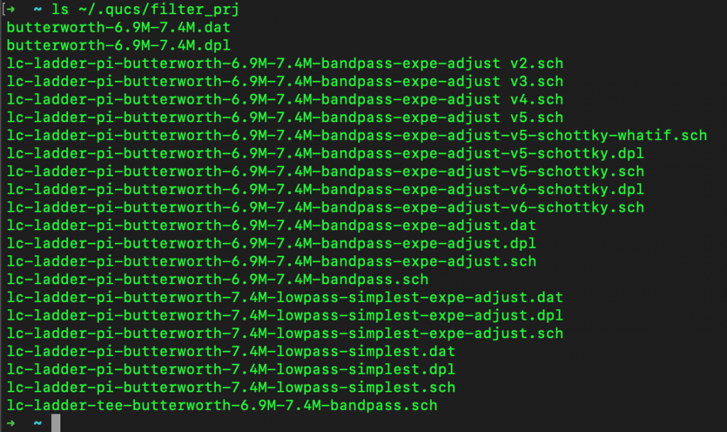
It corresponds actually to the folder ~/.qucs/<project_name> directory under which you’ll save all your schema files (*.sch). Creating the project directory will prevent some runtime errors when running simulations. Go ahead, create one and work there.
Then you go to Menu > Tools > Filter Synthesis:
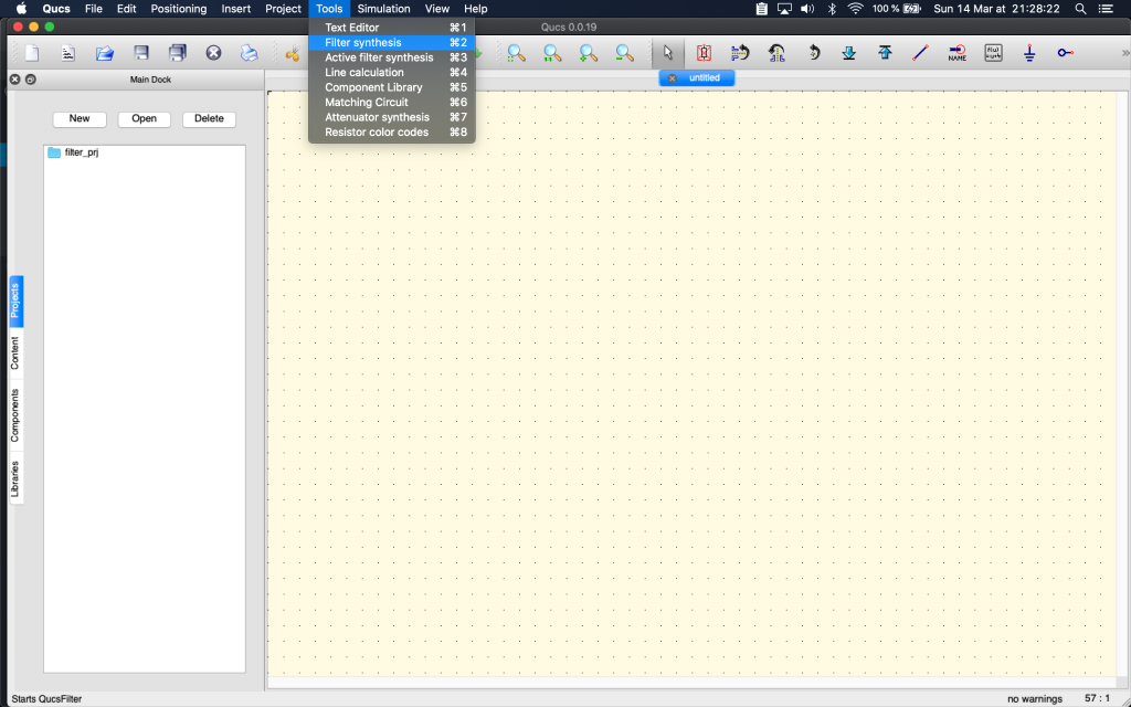
Qucs Filter is then run, but same thing as QUCS run, also often stays in the background. You’ll have to press ALT-TAB or Command-Tab to change window focus to it.
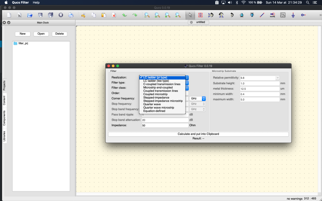
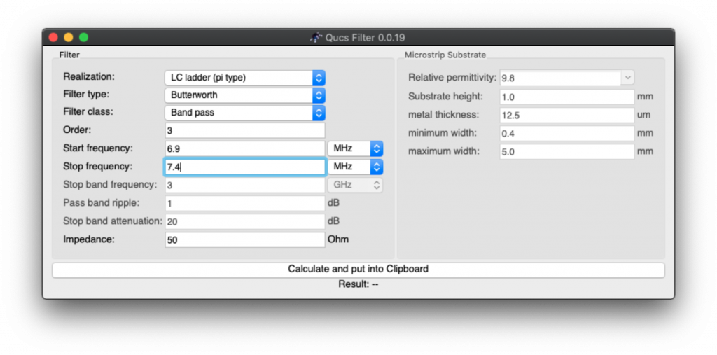
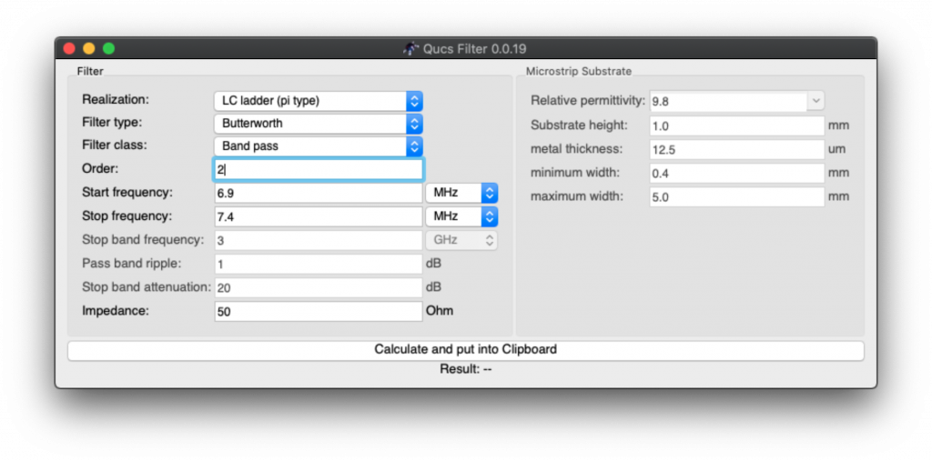
We choose LC Ladder (PI Type). Why? No idea. Suggestions are welcome. (In reality we rummaged through many web pages and many QUCS choices, comparing resulting filters with the simplest designs that were shown on the Net, before settling on this choice). Suggestions (and rationale) are really welcome about this.
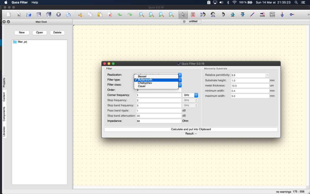
Then we change default type (Bessel) to Butterworth as it seems also to be a recommended LC type filter. (lessons learned not to use a RC filter and avoid signal power drops).
Then change default from Low Pass to Band Pass, and adapt start and stop frequencies, allowing for some “buffer space” around desired frequency.
Why this buffer space? because we’re going later to tweak values of electronic components to adjust with what we can easily buy, and therefore this will have an impact on the resulting frequencies that are allowed (that “pass”) or that are attenuated. Hence the choice to have some space around the 7 MHz HAM band frequencies.
The good thing is that the process described here works for all bands, you just need to adjust the values we’re specifying here. So if you want to build a filter for other frequencies, you can use this method and free software.
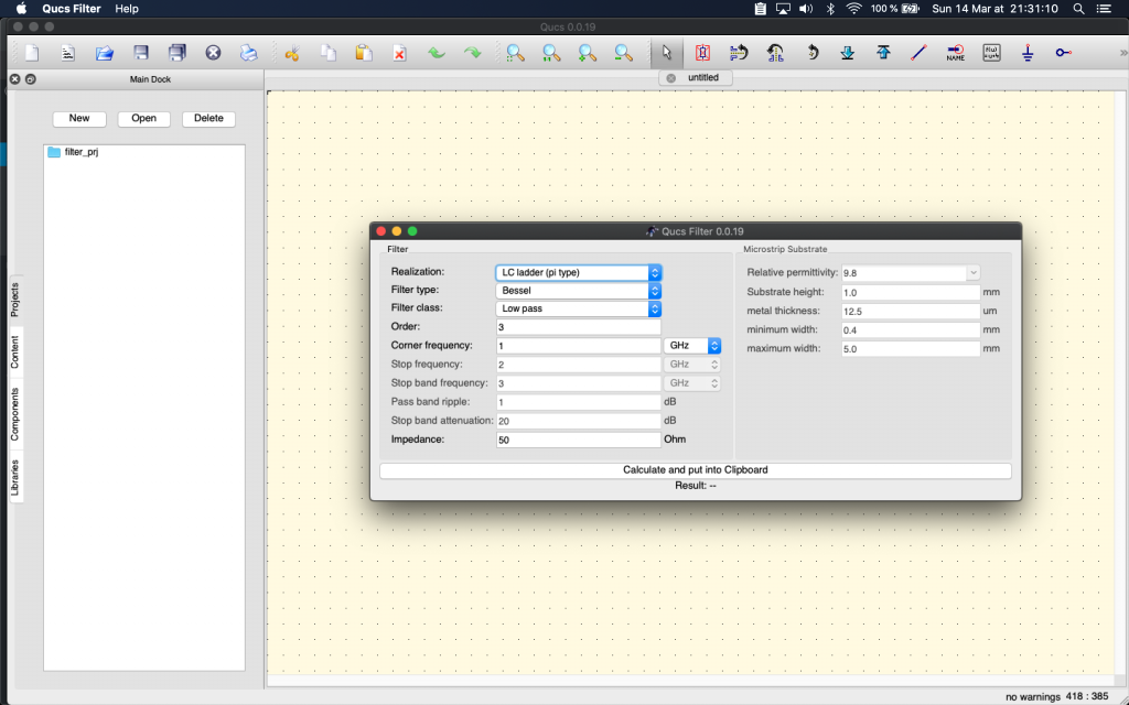
Here QUCS Filter with selected filters options and the frequencies input in MHz (note we changed the default frequency unit from GHz to MHz):
If you think nothing happens, well… you’re part right. It copied “something” (the result of filter computations) in the clipboard… then you need to switch to QUCS… and paste there in an empty circuit schema (Control-V or Command-V). A circuit skeleton will appear under your mouse cursor and hover on top of the schema for positioning of the filter result. That’s QUCS UX (User eXperience):
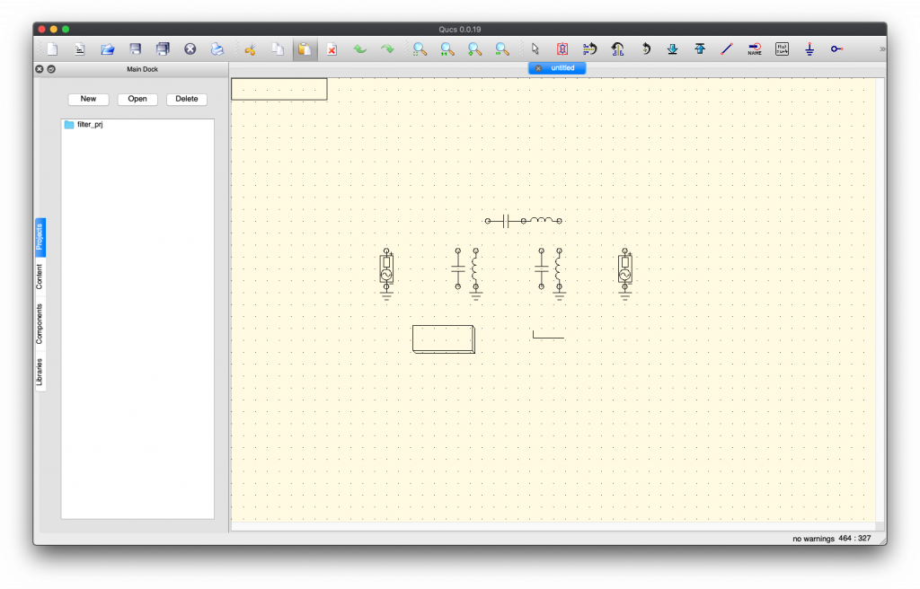
Move your mouse pointer to where you want your filter schema and click (Normal left click) to position it where you want on your page:

But if you continue moving your mouse, you’ll see that a copy of the filter is still selected, appearing as a skeleton (and can again be applied):
Yes… this is troubling UX. Just press ESC to deselect it (or “forget” it), it’s ok, one copy is enough and it is already there on your schema.
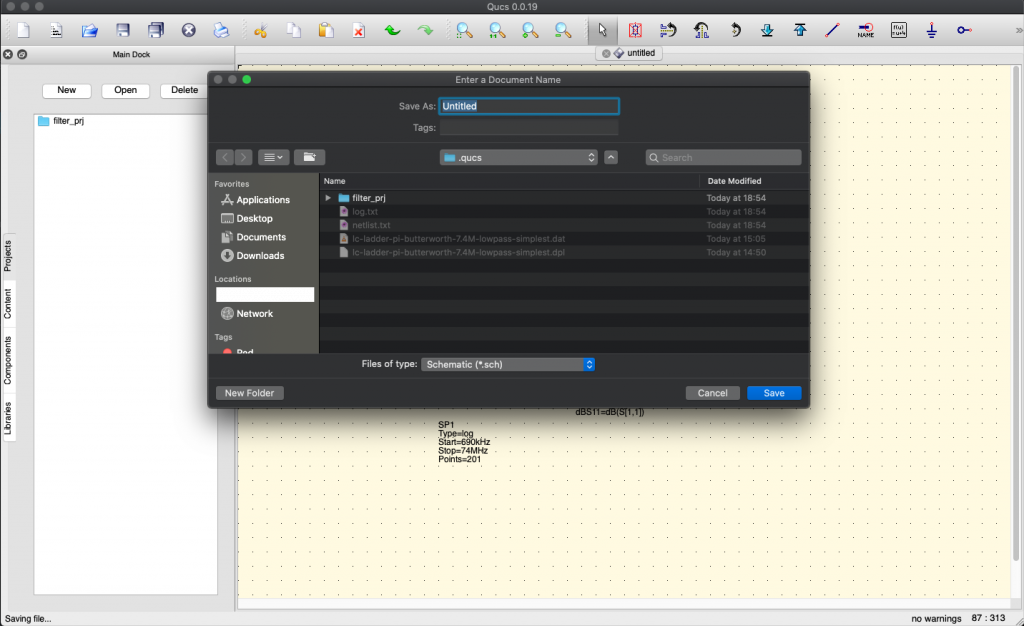
You can go ahead and save this:
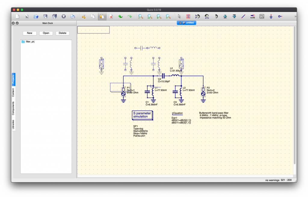
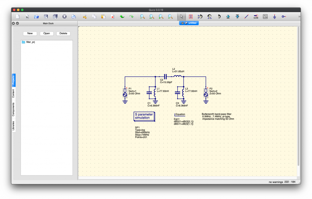
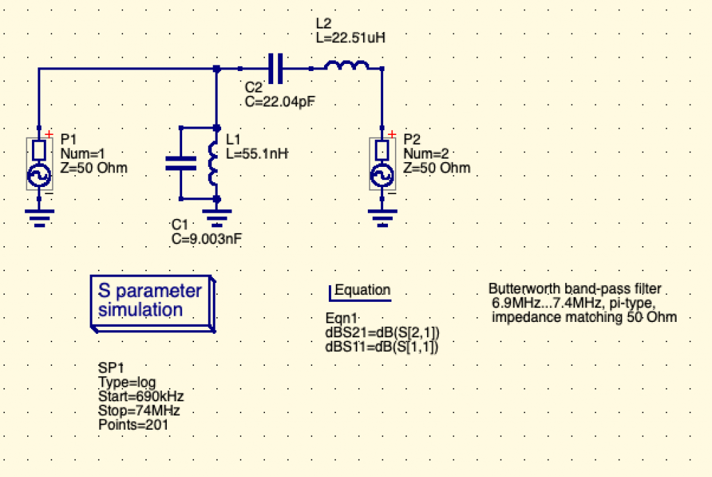
Please note that we choose to limit the amount of electronic components in the final circuit schema by selecting in the QUCS filter not “Order = 3” but to “Order = 2”:
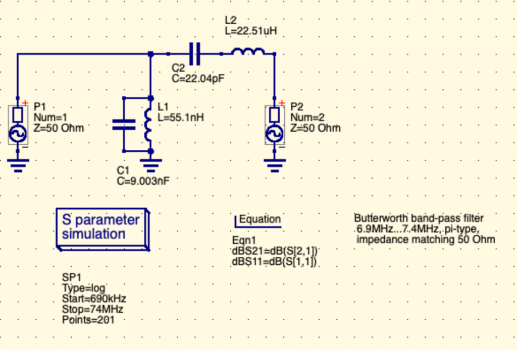
Resulting in this simplified schematics (with less electronic components):
We don’t know really the impact of such choice, so don’t hesitate to tell us. It looked like the only visible impact (visible during simulation) was that the filtered signal would go closer to full values (1x the passed signal, 0x power of filtered values) with order=3, which means that our choice of order=2 means that the filtering nor the pass-through will be complete. That means that a small attenuation of the allowed band would still be applied by the circuit. It means also that the filtering would be less “selective” than and third-order circuit. It’s not so bad since at these very low power (RPi outputs only in the mW range), the attenuation of these very lower spurious signals is really sufficient and would not radiate enough to be a real RF interference to other radio spectrum users. Please tell us if we’re wrong!
As we understand this schema:
- P1 (Port 1) is the generator, that is the TX output, the transmitter output:
- In our case the transmitter output is RPi GPIO output pin (GPIO4 or GPIO18 depending on software used on the RPi).
- Please note that it may be confusing as you see sometime “TX” label on some electronic schema for the input of the filter. It should be labeled “From TX” or “TX Output”.
- P2 (Port 2) is the antenna (ANT).
- It is also called sometime the “load” as you can output the radio signal to a resistive load to simulate an antenna (and avoid frying transmitters if they’re powerful enough and not connected to any “load”).
- It’s very useful during design as it prevents badly designed filters from emitting real RF to an antenna.
- Consider this when you start.
- The antenna is really the output of the filter.
A little reminder on electronic components
Electronic components on a schema are prefixed by a letter that indicate the type of component, and then a number that indicates its identification on the schema and the value of such electronic component.
Let’s see common type of electronic components used here:
- L: Inductors or Coils (“Bobines” or “Inductances” in french), these “store” energy as magnetic energy and give it back to the circuit.
- There are many inductors types, most of the time these are coils of copper wire around a metallic ring “core”.
- These are often used in transformers and amplifiers such as audio rigs, old power transformers, etc..
- Some types are looking like resistors (one ceramic package traverse by a wire that is exposed on both sides)
- C: Capacitors (“Condensateurs” in french), these “store” energy as electricity field energy and give it back to the circuit.
- R: Resistors (“Resistances” in french), these pressure and limit the passage of electricity in a way that changes the Voltage (“E” in english, “U” in french) and Intensity (I).
- There should be no specific resistor in filter circuits because resistors resists (!) and doing so, they heat up.
- The heat is actually radio signal power that dissipates.
- I.e.: the filter makes the whole radio signal power a bit weaker (or a lot weaker)
- The look of resistors (one ceramic package traverse by a wire that is exposed on both sides) is very common. It’s often called the “through hole” packaging, since now there are surface mount (SMD) versions of it.
Let’s simulate now our new filter !
Now we have a filter, let’s see how it behaves in front of input frequencies. Nothing is better than a graph to “see” your filter. Here is how to generate this filter graph through simulation.
We click on Menu > Simulation > Simulate (or type F2):
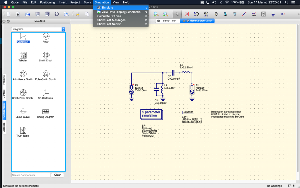
A new screen appears… But nothing happens: no simulation result.
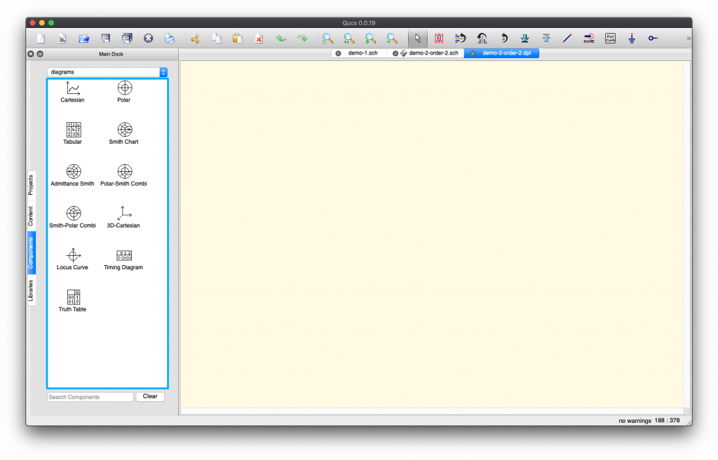
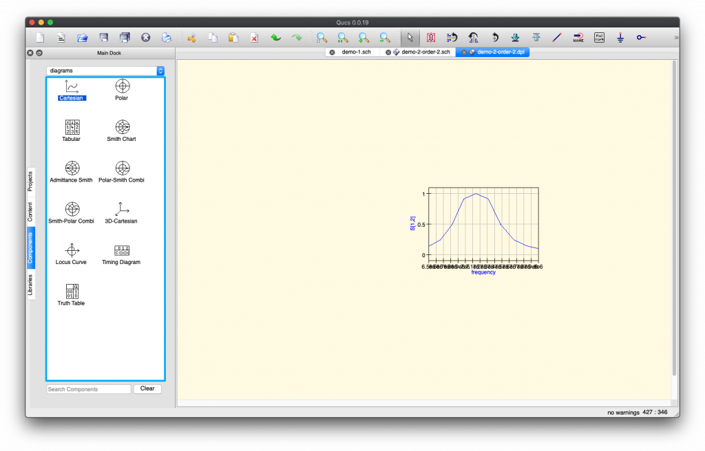
This is normal, QUCS is just waiting for you to chose which kind of simulation result you want to see. We’re going to chose Cartesian representation diagram, but the most elite radio guys will choose Smith (cuz it looks so cool! kidding aside, it must be awesome but it’s easier for newbies like us to read the simple graph):
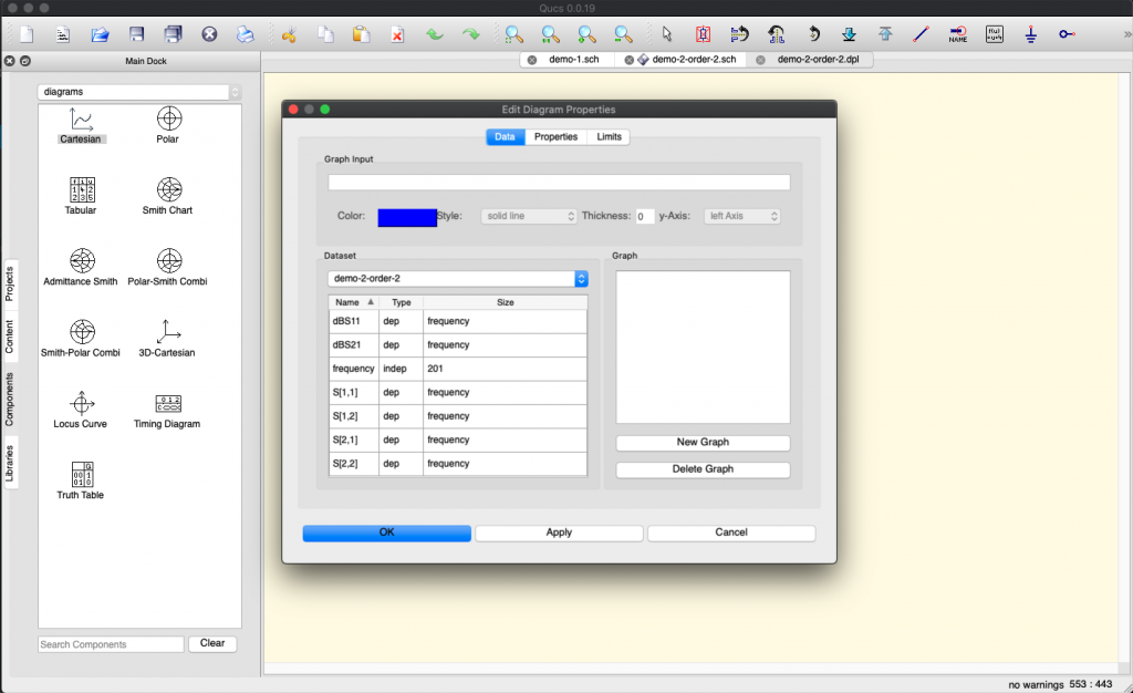
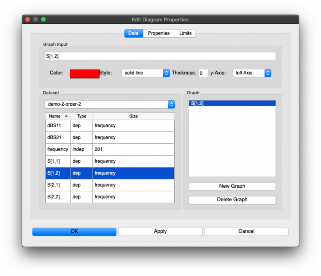
Now you need to set a few things for the simulation to run and result to appear.
First you need to say which signals you want to be graphed. Here what we understand is that S[1,2] is the filter output signal (i.e. the filtered signal). So we’re going to double click on S[1,2] to add it to the Graph:
But it’s not finished, we now need to restrict the Limits of the graph to only the portion of the simulation we’re interested in. So Click on Limits, Select Manual input for x-Axis:
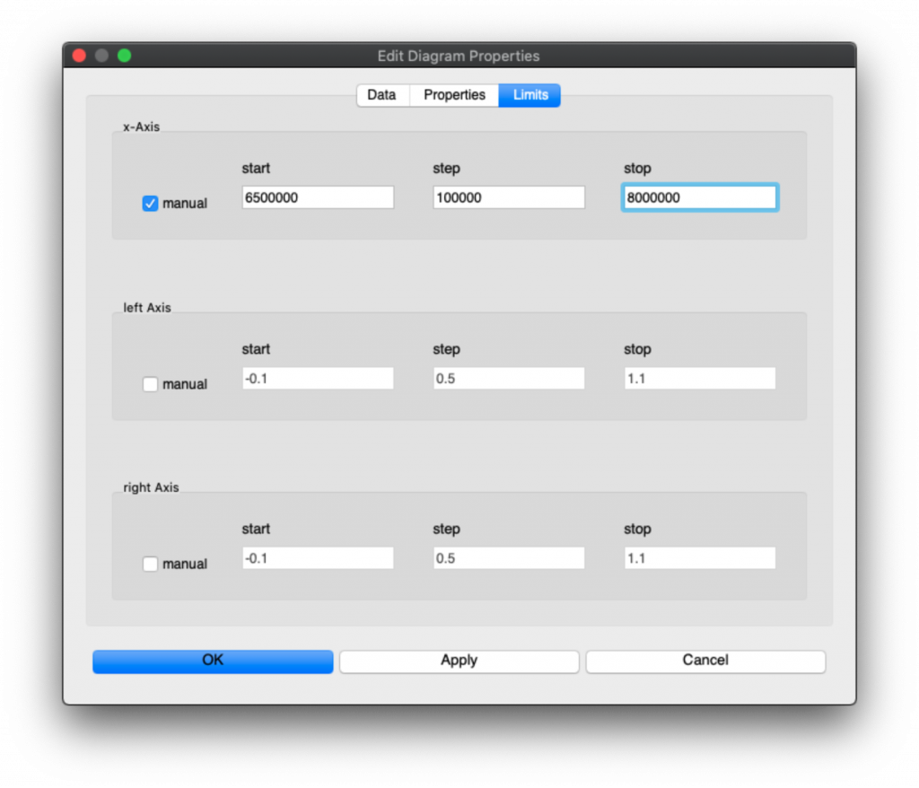
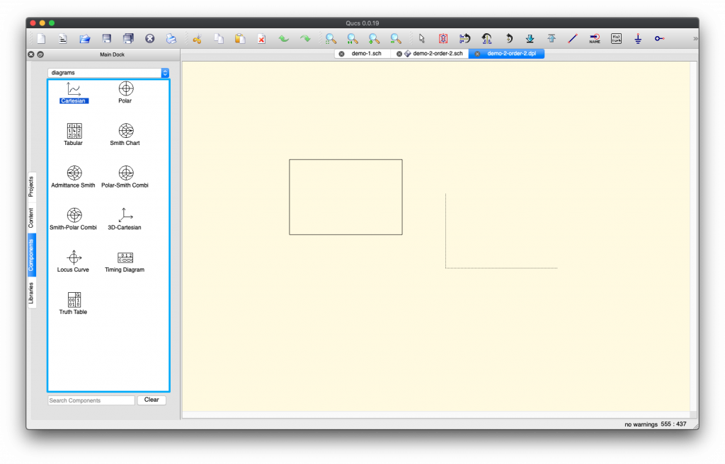
Then click “OK”. You’ll see a tiny graph appear.
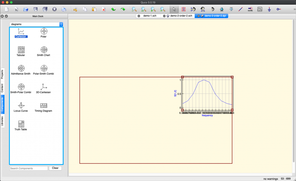
You can drag the corners by clicking into the graph and select one corner to drag in order to enlarge the graph:
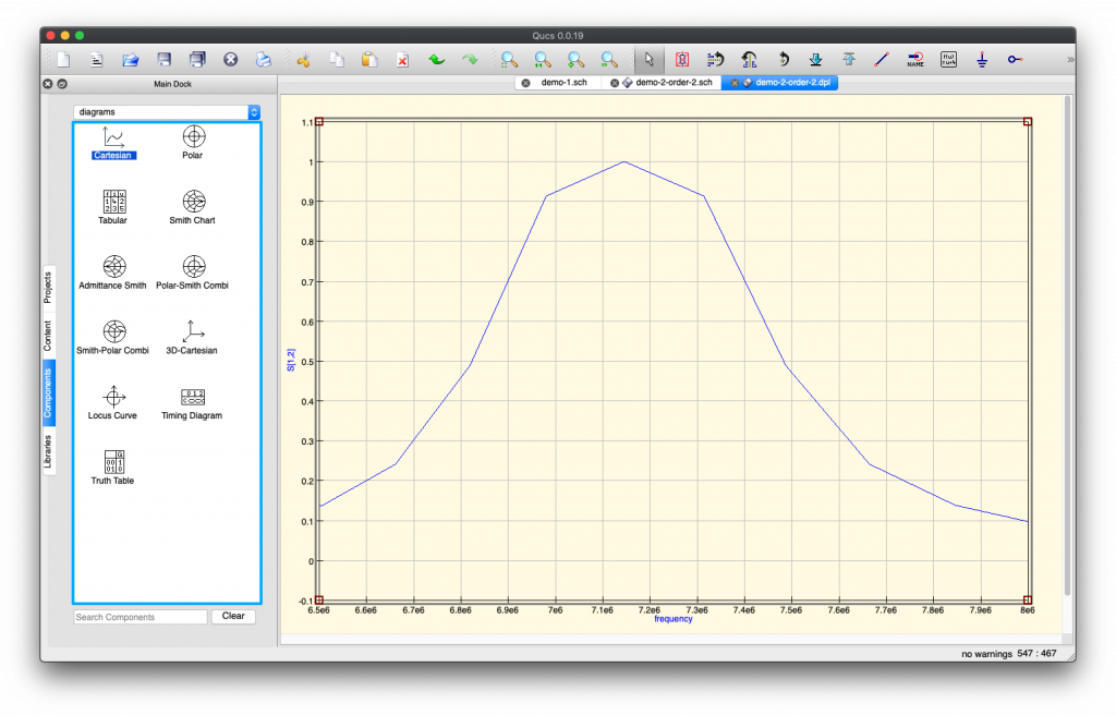
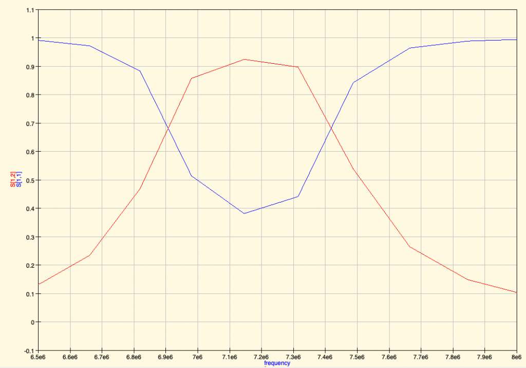
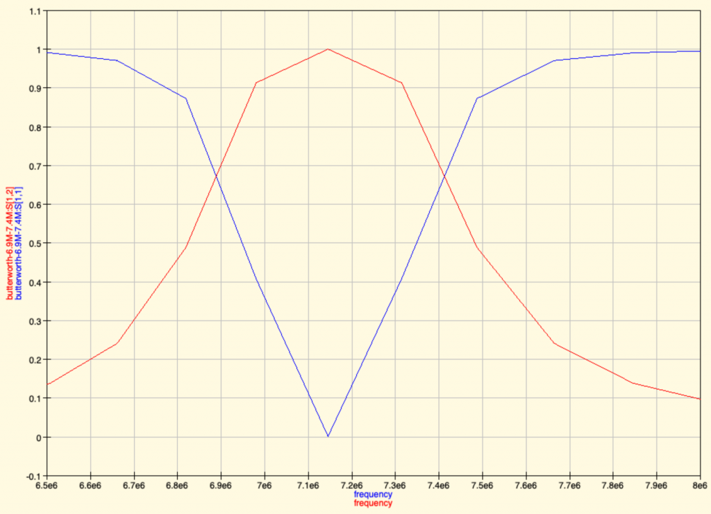
Then you have a nice result where you see in which frequencies your filter let’s the maximum of the signal go through:
Now we need to adjust the components
As you’ll see, the values of components are not standardised values, and we need to change some of the components values to match what we can find in shops.
So we’ll do one change, save, run a simulation and check that the effect on the filter is not so bad. Not so bad effect means:
- The filter still filters approximatively the same frequencies (same cut-offs)
- The filtering level is still the same (around 0.1x of the signal or better)
- The allowed (passed) signals are still around the same levels (0.9 or better)
So the raw values we had without adjustment of electronic components were:
Here is the adjusted graph we end up with:
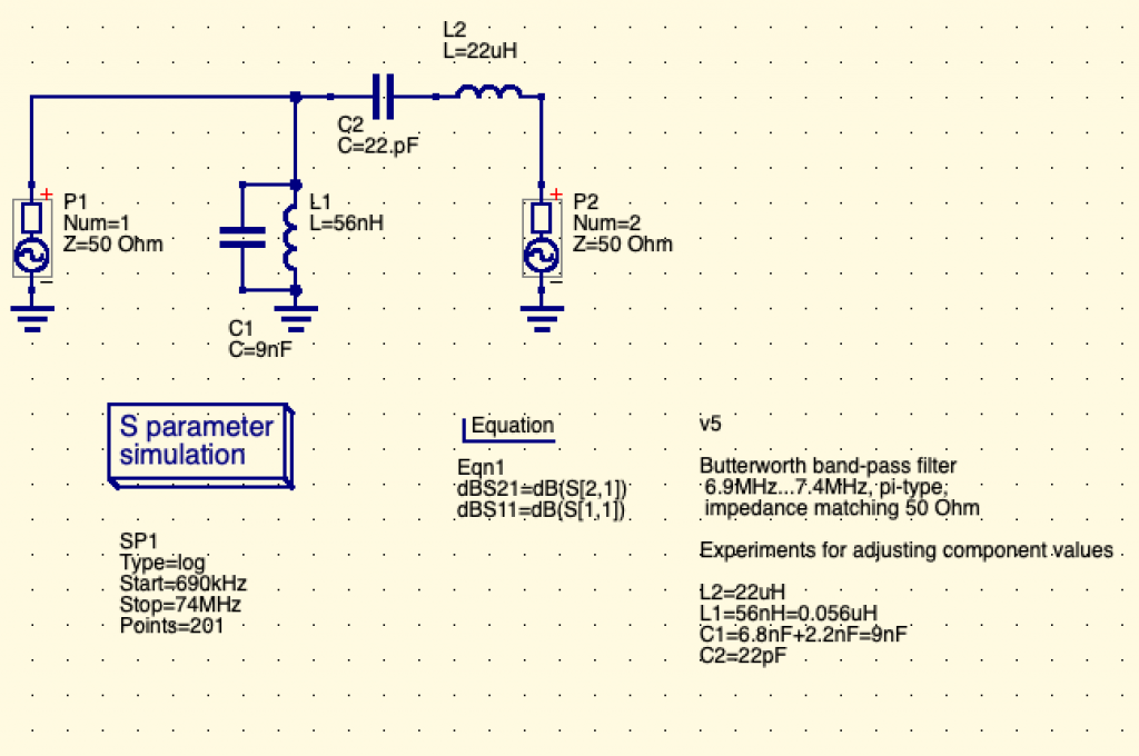
And the corresponding filter simulation output:
Now this is probably not how we should be building filters. And we’re open to suggestions or links to good resource to learn how to do better. It’s for sure not the Electronic Engineer’s way and we’re eager to do better.
Protect the RPi: Schottky Diode
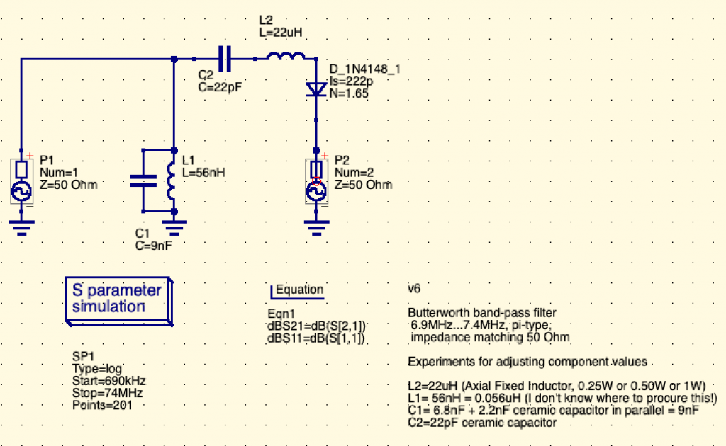
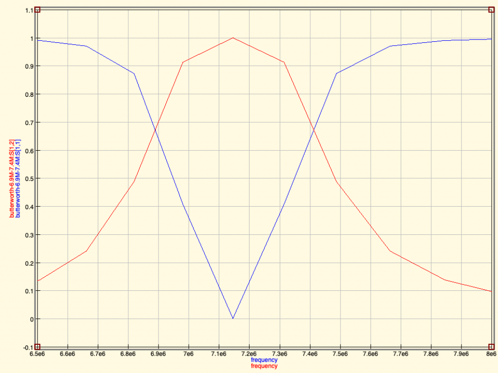
We heard (and felt with our fingers) that antenna can collect some static electricity, and that we may need to protect the RPi against such electricity using a Schottky Diode. Although not classified as Schottky Diode, the 1N4148 signal diode was often quoted as the way to go to protect our RPi. So here we go and added to the schema:
Then we proceed to simulate again to check the resulting graph:
We see that the filter’s output seems ok.
Now that’s where we are for now. The schematics are here.
Update for off-the-shelf capacitor values
For completeness, here is the v7 with the split C1 capacitor to reflect reality of capacitors values that are easily available in shops:
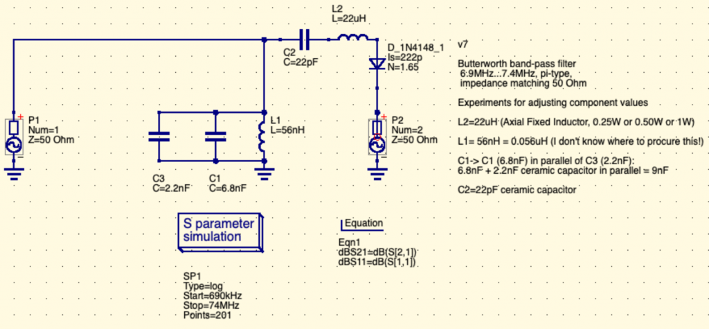
And the resulting simulations gives the same result:
Feedbacks and comments
We’re eager to hear more from you if you have any question or feedback. Please either come to /tmp/lab Matrix chat room: #tmplab:matrix.fuz.re or comment on the reddit link (that will be posted in some time). We also expect to make a short video too to show people how we use QUCS for this.
Next episodes:
- Building the filter: soldering, components, testing
- Antenna connections and measurements with NanoVNA
- Setting up antennas, safety considerations, emitted power
- Building our next antenna(s)
- Testing the reach of WSPR weak signals
In the meantime, kind regards and please, come and participate. There are no stupid questions. There are no bad feedbacks (but please be kind 😉 ).
Feedbacks and discussion
Ah… that’s awesome, the power of internet community, already just a few minutes after publishing some kind souls gave comments about the design and very informative resources, so I’ll take them point by point here.
Feedback #1: LPF
I would have used a low pass filter, not bandpass.
Yes, we tried some LPF (Low Pass Filter) designs and failed at getting a nice output (the cut-off was very slow and the levels not great). What kind of LPF would be best for this application? (as indeed it sounds like a good candidate)
Here is a LPF design (along the lines of what the links below advised):
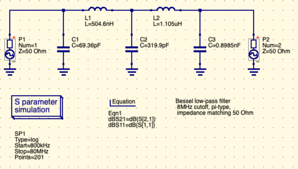
And then the simulation results (here we use dBS11 and dBS21 data lines to plot relative power drop in dB. Have a look at this table to understand the relationship between dB and power multiplier. To remember easily, +3dB is double the power, -3 dB is half the power. +6dB is 4 times the power, etc..):
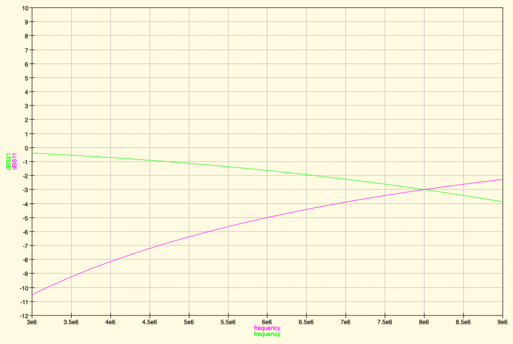
What I subjectively find is that the cutoff frequency isn’t very “sharp” in simulation (supposedly it’s sharper in reality), and with the same amount of electronic components as a Band Pass Filter (BPF). Not sure what the benefit of the LPF would be.
What do you see if you model your filter at 2x and 3x the working frequency?
Here is the simulation result of our BPF (Butterworth Band Pass Filter) with very wide band, not sure that’s what was asked:
Feedback #2: Diode as harmonics source 🙁
Also not sure you should have the diode protection. Diodes cause harmonics so as quickly as you try to filter them you have placed a device to create more 🙁
Hmm…. how to test for this? Would the simulation show such harmonics Indeed it will be easy to test in reality.
It’s easy to add or take off anyway in the resulting circuit.
Feedback #3: References on how to do it right
Maybe take standard values for low pass filters from webpages like http://www.gqrp.com/technical2.htm then change the inductance values to the nearest standard value fixed components?
Definitely, the PDF ressource in the GQRP link is excellent and gives a practical and nice table of values for all significant HAM bands (frequencies).
The Capacitor symbol seems to indicate that it’s polarized capacitors that are used. Any feedback how important it is to use polarized capacitors here?
The band table values for components gives also the commercially available component values:
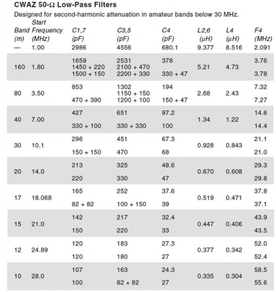
Go read the original PDF for more details.
Also some nice ARRL article about the CWAZ filters mentioned in the above resources.
Reading about these filters the CWAZ filters advised by GQRP seems to be advised because of the inadequate filtering of Chebyshev LPF when power levels greater than 5W (FCC requires transmitter spurious outputs below 30 MHz to be attenuated by 40 dB or more for power levels above 5W)
In our case, the power levels are far less than 5W, so actually we could maybe use a simple Chebyshev 3rd order Low Pass Filter and that could be good enough. The filter synthesis result of such LPF could be as simple as:
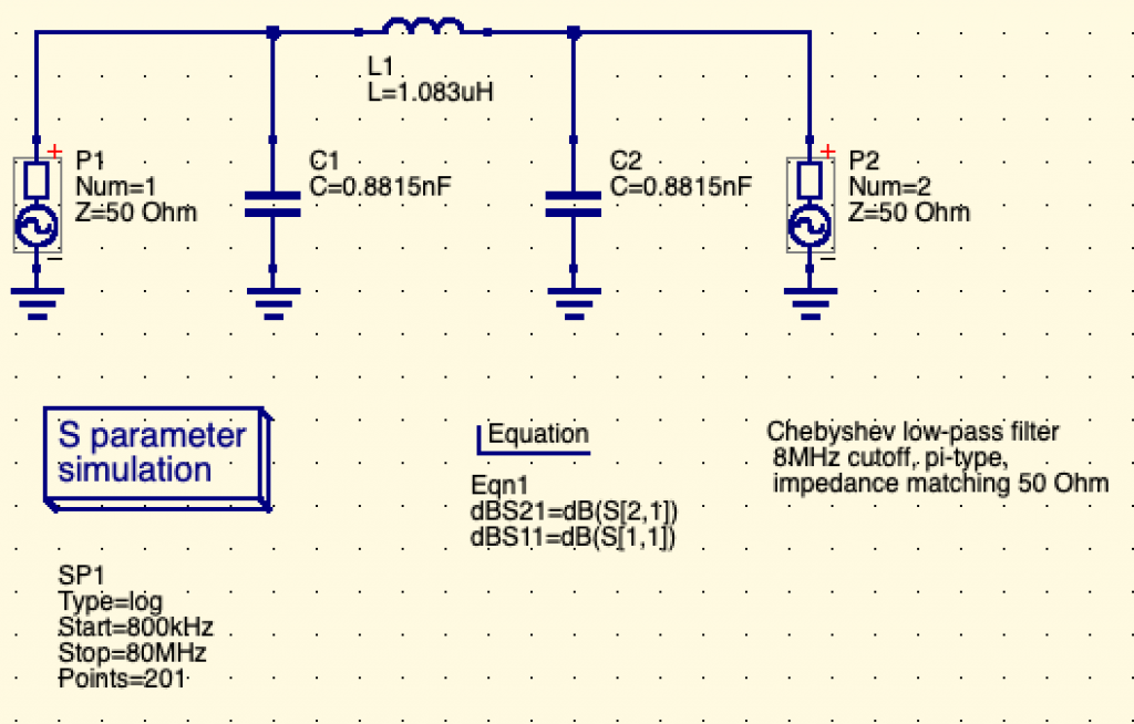
With resulting filter simulation:
Now when we adjust to available component values, this gives:
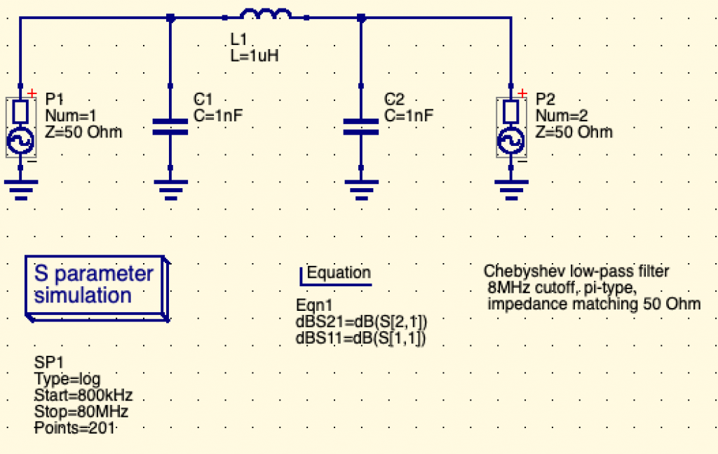
How simple, 2x capacitor of 1nF, 1 inductor of 1uH. Now we’ll see if this fairy tale matches the reality of what we need once implemented 😉
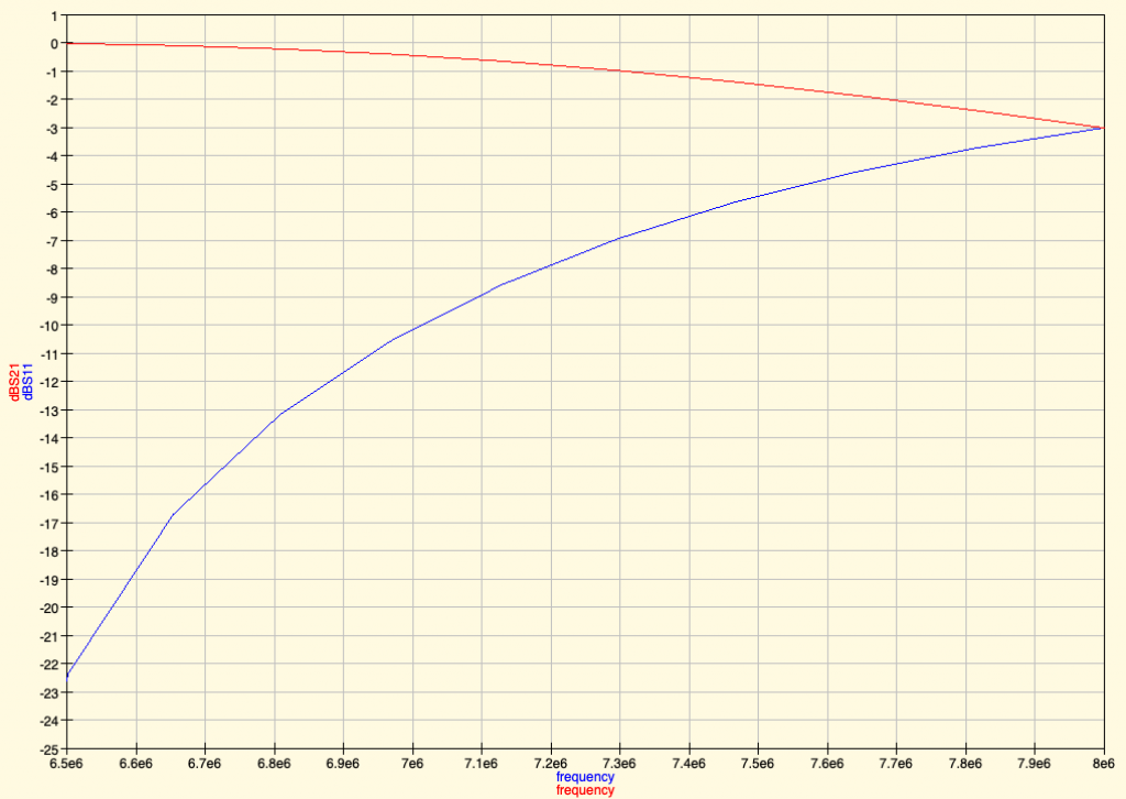
It simulates to:
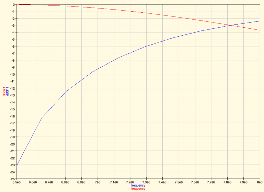
Which seems pretty much acceptable. Do you think the same? Tell us.
Feedback #4: Filter may not filter enough at higher frequencies
The filtering of our simple filters may not be enough: the roll-off, that is the drop after the cutoff frequency, may not be steep enough.
Filters use often multiple “poles”, that is multiple Inductor+capacitor “legs” to the ground, in order to filter more (e.g. to -60dB or more) at higher frequencies. The more poles (the “higher order” filter), the steeper roll-off, the more attenuation of signal at higher frequencies.
More filtering means less spurious frequencies. And that is the goal of a better filter. Indeed, that’s the role of the CWAZ filter.
Note that Chebyshev filters use order 3, 5, 7 (odd numbers) only when doing filtering synthesis of a passive filter (i.e. one that you don’t need to supply external electricity power supply to work).
So that means that we may either try such filter synthesis…. or use the CWAZ filter that is quite simple still.
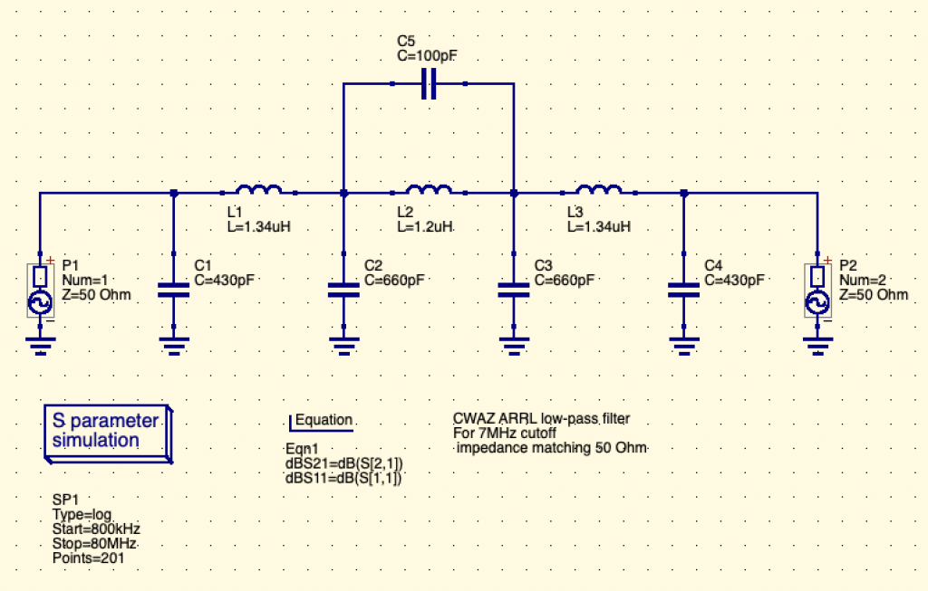
Now the problem is to try to use very standard values for electronic components.
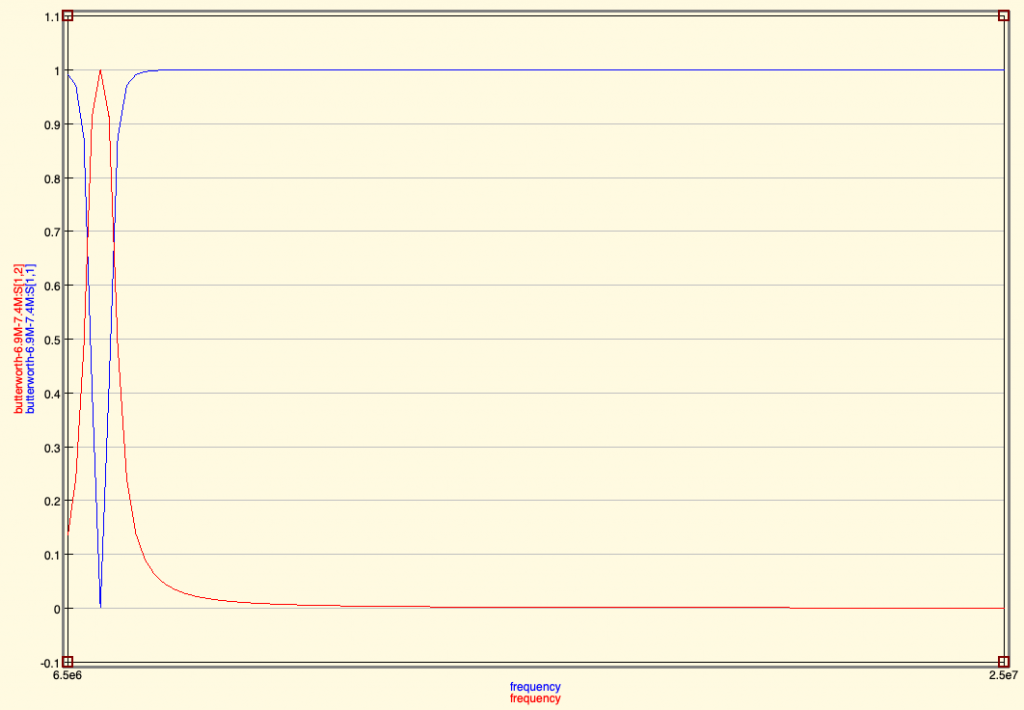
Here for 7MHz, it’s a bit easier as 430pF is 330pF (standard) + 100pF (standard) in parallel. And 660pF is two 330pF capacitor (standard) in parallel.
The resulting filter graph is actually very good:
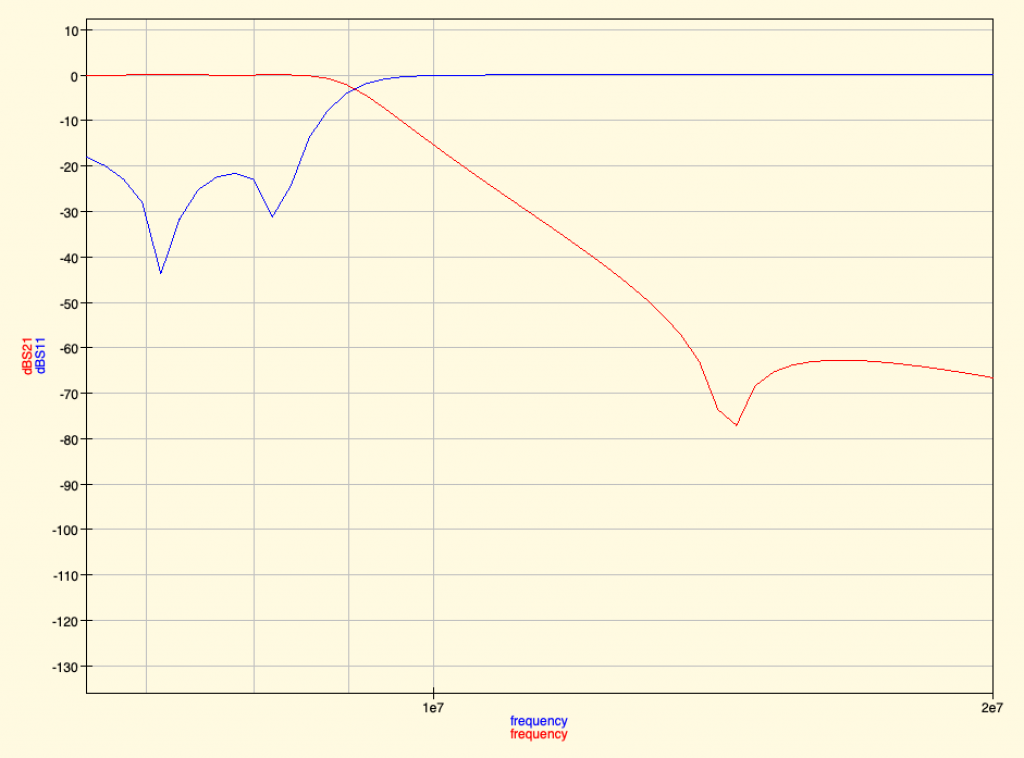
1e7 = 10 MHz. 2e7 = 20MHz, so we see that around 9 MHz the signal starts to be filtered. And that a -70dB filtering means the power level was divided by 10 million 🙂
The inductor value of 1.34 uH is not at all easy to find in already prepared packages. If we replace this 1.34uH inductor by a 1.2uH inductor, there’s a risk for a mismatch impedance (meaning your antenna may reflect back some part of the signal to the raspberry pi and damage its circuit components). Ahh… so either we don’t filter enough or we risk having reflected signal from the antenna to the transmitter. What a wonderful world 😉
Future
The new plan is to try to build both our first DIY designed Butterworth BPF filter, the CWAZ and the LPF Chebyshev filter and evaluate these.
We’ll improve this article when finished studying these ressources! Thanks to everyone who is providing feedbacks and ressources!
Thank you
Thanks to the following awesome people who helped either with Radio or with the resources to post and document this exploration:
- G0DUB
- Alban
Ressources
Some ressources that may be useful regarding this post:
- http://rockingdlabs.dunmire.org/exercises-experiments/bpf-analysis#TOC-Universal-Dual-HF-Band-Filter-BPF-
- https://tapr.org/product/wspr/
- https://github.com/JamesP6000/WsprryPi/blob/master/README
- https://github.com/dslotter/HamPi
- https://hexandflex.com/2020/01/11/impedance-matching-with-qucs-studio-and-vna/